
“We describe a model of perceptual inference in primary visual cortex (V1) equivalent to a minimal diffusion model whose function can be readily understood from its parameters.”
— Yun et al., 2026
It is tempting to think of the primary visual cortex (V1) as a deterministic feature extractor. Light hits the retina, spikes travel down the optic nerve, and V1 meticulously catalogues edges, orientations, and spatial frequencies. Yet, visual perception is fundamentally an act of inference. When faced with an occluded object or a dimly lit scene, the brain does not simply freeze; it actively reconstructs. This process requires dealing with ambiguity, filling in the gaps with prior expectations.
For a long time, standard feedforward artificial neural networks struggled to capture this generative aspect of biological vision. They provided excellent classifications but poor reconstructions under extreme noise. But recently, a specific class of generative machine learning — diffusion models — has shown an uncanny ability to denoise and construct coherent images from pure static. A recent preprint by Yun, Belsten, Bi, Kadkhodaie, Chen, and Olshausen (2026) [1] offers a substantive, testable hypothesis: the recurrent dynamics of V1 can be understood as a minimal diffusion model. It is a genuinely exciting development. It is also more complicated than that™.
The context: ambiguity and recurrence in the visual cortex
To understand why this connection is intriguing, we must look at the constraints of perceptual inference. Consider you are walking through a dense forest at dusk. A shadow moves. Your brain must immediately infer whether it is a branch or a predator. You have limited, noisy sensory input. To solve this, your visual system relies heavily on horizontal connections within the superficial layers of V1 [2]. These connections link neurons that share similar orientation tuning across different parts of the visual field.
Previous models have successfully described V1’s responses using sparse coding principles [3], which suggest that the brain represents images using a small number of active neurons at any given time. Sparse coding represents an image $\mathbf{x}$ as a linear combination of basis functions (or receptive fields) $\boldsymbol{\Phi}$ multiplied by a sparse set of latent activities $\mathbf{a}$:
\[\mathbf{x} \approx \boldsymbol{\Phi} \mathbf{a}\]The objective is typically to minimise the reconstruction error while enforcing a sparsity penalty (like an $L_1$ norm) on the latent activations.
\[E = \frac{1}{2} || \mathbf{x} - \boldsymbol{\Phi} \mathbf{a} ||_2^2 + \lambda ||\mathbf{a}||_1\]However, standard sparse coding assumes the latents are independent of one another — a factorial prior. That is the real gap, and it is worth being precise about what it is not: sparse-coding inference is already iterative, and with an $L_1$ penalty it denoises perfectly well. What it lacks is any way for one feature to lend support to another, which is exactly what you need if a half-occluded edge is going to be completed by its neighbours. We need a model whose prior carries the co-occurrence structure of the world, and which can use that structure to pull a noisy input back towards a natural image manifold.
What that looks like is easier to show than to describe. The display below is built in the manner of the contour-integration stimulus of Field, Hayes and Hess [5]: a smooth path of oriented elements buried in a field of randomly oriented ones.
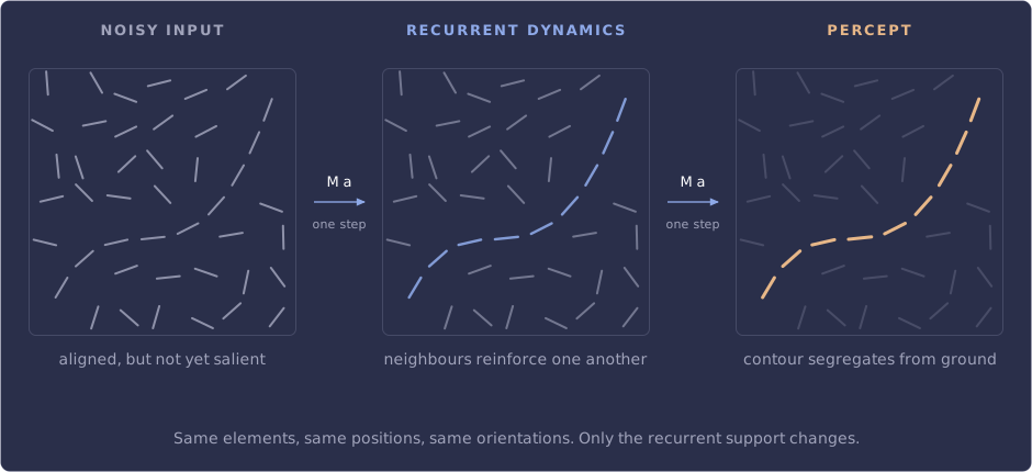
The three panels are the same image. Not similar — the same: every element sits in the same place at the same angle throughout, and the nine on the path were aligned from the start. Nothing is added, nothing turns, no fresh evidence arrives. What changes is how much recurrent support those nine receive from one another, and that alone is the difference between a field of clutter and a contour you cannot unsee. The gap between what is in the input and what is in the percept is the work inference does.
The technical core: V1 as a denoising score matcher
The paper by Yun et al. proposes an elegant extension to standard sparse coding to solve this exact problem. They give the latents a prior that does not factorise — one in which the variables are permitted to depend on each other — carried by an unconstrained matrix of pairwise interactions, denoted as $\mathbf{M}$. This allows them to formulate perceptual inference as a recurrent dynamical system, unrolled as a sequence of proximal updates run to a fixed point.
Instead of just penalising independent activations, the model introduces an energy term that accounts for how different features (like collinear edges) co-occur in the natural world:
\[E_{prior} = -\frac{1}{2} \mathbf{a}^T \mathbf{M} \mathbf{a}\](The paper writes this term with the opposite sign inside an energy it minimises. I have flipped it so that a positive entry in $\mathbf{M}$ reads as excitatory throughout, which makes the figures below easier to follow.)
To train this model, they employ a denoising score-matching objective [4]. This is the same fundamental principle underlying the diffusion models behind modern image generation. Instead of explicitly defining a loss function to reconstruct a clean image, the model learns to estimate the gradients of the data distribution — the “score” $\nabla_{\mathbf{x}} \log p(\mathbf{x})$.
The network learns to take a noisy state $\tilde{\mathbf{x}}$ and push it slightly towards a more probable, natural-looking state. In pseudocode, a simplified version of this inference process over time $t$ might look like this:
# Pseudocode for perceptual inference as a recurrent process
def infer_percept(noisy_input, M, Phi, lam, num_steps=100, dt=0.01):
    # Latents start at zero, as in the paper's ISTA formulation
    a = zeros_like_latents()

    for t in range(num_steps):  # in the paper, iterated to convergence
        # 1. What the current reconstruction still fails to explain
        residual = noisy_input - Phi @ a

        # 2. Feedforward drive, plus recurrent horizontal support via M
        drive = Phi.T @ residual + M @ a

        # 3. Gradient step, then the proximal step: sparsity plus rectification
        a = relu(a + dt * drive - dt * lam)

    return Phi @ a
When the researchers trained this minimal diffusion network on natural images, something worth pausing over occurred. The learned interaction matrix $\mathbf{M}$ came to look like V1’s horizontal connectivity: strong positive interactions between latent variables representing collinear, similarly oriented edge features. If a vertical edge is detected here, a vertical edge slightly above it is highly probable, so the weight between them becomes strongly excitatory.
Two separate bodies of work are worth keeping distinct here, because the model touches both. Gilbert and Wiesel [2] established the anatomy: horizontal connections in superficial V1 preferentially link cells of similar orientation preference. Field, Hayes and Hess [5] established the behaviour: human contour detection acts as though it uses what they named an association field, a rule about which neighbouring elements reinforce one another. The two are usually assumed to be the same thing seen from different angles, and that assumption is reasonable, but it is an assumption. What the model contributes is a third arrival at the same layout from neither anatomy nor psychophysics, but from the statistics of natural images.
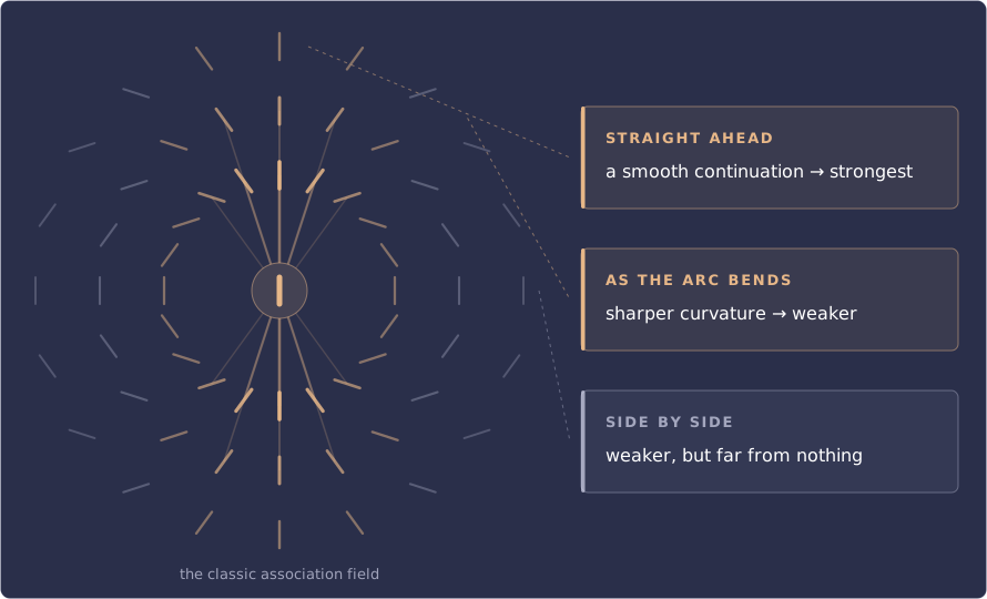
The association field as the psychophysics describes it: a neighbour helps you see a contour in proportion to how gently the path joining it to the centre has to bend. Straight ahead helps most, and the help weakens as the arc tightens. It does not simply vanish at the sides, though, and this is where the figure is easy to over-read. In their Experiment II, Field, Hayes and Hess turned every element ninety degrees, square to the path it lay along; so long as the path itself ran straight, both observers still found it, at 0.79 and 0.89 correct against a 0.5 baseline. Both angles matter, though, and they are not the same angle. Turned square to the path, detection had fallen to chance by a 45-degree turn from one element to the next; left aligned along it, observers stayed above chance out to 60. Only one of those two is the angle the figure varies. So across the range where the effect survives at all, what changes is the strength of the facilitation rather than its presence, and nothing in their data reverses into active suppression. Suppression is a stronger claim than Field, Hayes and Hess anywhere make, whatever the figure is often remembered as showing. And the model reproduces the facilitation half of this from natural image statistics alone, which is the striking part. Its inhibition works differently: $\mathbf{M}$ learns to inhibit itself hard, which is how it keeps the code sparse, and the inhibitory connections it does learn are more weakly orientation-tuned than its excitatory ones. Same excitatory geometry, arrived at independently; a different solution to keeping the representation sparse.
The denoising performance is strong too. The model restores extended contours amid extreme ambiguity, coming close to a black-box diffusion network in the generalisation regime — a qualifier worth keeping, along with the fact that the comparison network here is itself deliberately small. This is not a claim to have matched a production image model.
One detail the pseudocode above glosses over is worth restoring, because it is doing real work. The recurrent drive is not simply $\mathbf{M}\mathbf{a}$; the learned prior is scaled by a noise-dependent gain, so that as ambiguity rises the network leans progressively harder on the prior and less on the incoming evidence. That is the mechanism behind the whole “resolving ambiguity over time” story. Half of it falls straight out of the maths, since the $\sigma^2$ factor is just how the likelihood term is weighted; the gain applied on top of it, though, is a small learned network rather than something the derivation hands you.
There is also a pleasing lineage here that the paper does not draw attention to: Olshausen is a co-author, three decades after the sparse coding work [3] this model extends.
Implications: two-way traffic in NeuroAI
The reason this one is worth your time is that it pays out in both directions, which is rarer than the NeuroAI label tends to suggest.
For neuroscience: it converts a description into a prediction. We have known since Gilbert and Wiesel [2] that V1’s horizontal connections preferentially link cells with similar orientation tuning, and since Field, Hayes and Hess [5] that human contour detection behaves as though it uses an association field. Neither result tells you why the connectivity has that shape. Score matching offers a candidate answer: it has that shape because that is what denoising natural images demands. What makes this more than a nice story is that it is checkable. If the account holds, population activity during an ambiguous task should follow the particular gradient flows the trained $\mathbf{M}$ predicts, rather than merely settling into a cleaner percept by some other route. That is a real test, and I would like to see someone attempt it.
One word needs care, though. It is tempting to conclude that the connections are therefore optimal. The model is trained to approximate the score of the natural image distribution, so within its own assumptions it is doing the right thing by construction — and that is a claim about the model. Agreement between a trained network and an observed anatomy is evidence of a shared constraint, not proof of a shared derivation. Two systems can arrive at similar structure for different reasons, and frequently do.
For machine learning: the contribution is smaller than the framing around this kind of result usually suggests, and more useful for being smaller. It does not explain how a production diffusion model generalises. It shows that one diffusion model, built deliberately small enough to read, generalises by enforcing consistency among local image features through pairwise interactions — and because the network’s Jacobian decomposes directly in terms of $\mathbf{M}$, you can watch it happen rather than infer it from probes after the fact. Interpretability by construction rather than by autopsy. Whether anything similar runs inside a large model is open, and going to look for analogous structure in one is the obvious next move.
The result I keep returning to is the strangest one: over 30% of the units stop listening to the image entirely, forming a layer that enforces global structure instead of reporting on pixels. To the authors’ credit they do not merely note this, they ablate it — remove the detached units’ recurrent interactions and denoising collapses at high noise, with the network losing the long-range coordination that holds an image together. So these units are doing real work here. What is not established is whether the arrangement is peculiar to a small model with few latents to spare. If large diffusion models also devote a sizeable share of capacity to units that have stopped listening to the input, I would have to rethink what that capacity is buying. That is the fork I would watch.
Limitations
The model is a beautiful, minimal abstraction, and it leaves a good deal unresolved. Three gaps stand out, and they are not equally serious.
First, biological networks communicate with discrete spikes, whereas this model uses continuous rate variables. Spiking imposes a severe communication bottleneck and an asynchrony that a rate-based model glosses over. Real, but I suspect survivable: rate-based abstractions have earned their keep in V1 for decades.
Second, the model treats V1 and its horizontal connections in isolation. Perception leans heavily on top-down feedback from higher areas like V2, V4 and IT, which carry priors about objects and context. A shadow reads as a predator partly because of local edge continuity, and partly because you are in a forest at dusk. That the model does contour completion well without any of that is a genuine result. It also marks the ceiling: what it can settle are ambiguities resolvable from within the image itself — and it does reach across the image to do so, since the detached units enforce global consistency — but not ones that need knowledge of the scene the image is of.
Third, and this is the one that actually threatens the claim: the training procedure. The authors use implicit differentiation on a score-matching objective, which is an excellent machine learning technique and precisely the sort of thing we do not think cortex can do. So the model accounts for the form of $\mathbf{M}$ while offering nothing on how a brain could ever arrive at it. The paper does not raise this, which I think is the one real omission in an otherwise careful piece of work. It is the load-bearing gap, because the neuroscience claim is not “this connectivity is a good denoiser” but “cortex has this connectivity because it is a good denoiser” — and the second needs a mechanism the first does not.
That thread runs straight into the other post in this series. Dendritic Localized Learning comes at the same problem from the opposite end, asking what learning rules a neuron could actually run given only locally available information. Neither paper closes the loop. Read side by side, they mark out its shape.
Worth naming the premise underneath all of this, too: that the brain has no access to global gradients. That is an assumption the field has agreed to work under rather than a settled finding. I think it is a reasonable one. It is also doing an enormous amount of work.
What to watch next
Three things, roughly in the order I expect them.
Someone takes the prediction seriously and records from V1 during a contour task, to see whether population trajectories follow the flows the trained $\mathbf{M}$ implies. Spiking dynamics and top-down feedback get folded into the same framework, which is tractable and the natural extension for this lab or a neighbouring one. And, hardest of all, local learning rules that approximate a score-matching objective — the piece that would turn this from an account of what V1’s connectivity is good for into an account of how it got that way.
If I had to bet: the recordings arrive first and are messier than anyone currently hopes.
References and resources
[1] Yun, Z., Belsten, A., Bi, D., Kadkhodaie, Z., Chen, Y., & Olshausen, B. A. (2026). Toward a mechanistic understanding of inference in visual cortex and diffusion models. arXiv preprint arXiv:2607.15693.